
Numerical Recipes in Fortran
The Art of Scientific Computing Second Edition
http://www.mathtools.net/
The technical computing Portal
for all you scientific and enginenring needs
http://www.ddj.com/topics/scientific/articles/
Scientific Computing
edited by Jeremy Siek(jsiek@lsc.nd.edu)
http://www.cs.fsu.edu/~mascagni/papers.html
Dr. Michael Mascagni – Recent Papers
http://tonic.physics.sunysb.edu/docs/num_meth.html
Numerical methods
http://www.math.uic.edu/~hanson/mcs471/float_arithmetic.html
Floating Point Arithmetic Notes
For MCS 471 Numerical Analysis
| Software | O.S. | Language |
|---|---|---|
| Octave | Linux / Win | English |
| Matlab | Win | English |
| Scilab | Linux / Win | English |
| Software | Size |
|---|---|
| Octave for Windows | 9,47 MB |
| Turb Pascal 7 | 1,74 MB |
| Scilab26 | 9,76 MB |
Manuals
More information
Other suggested links
MATLAB
Try this Link for more MATLAB infos…
Click on website
The MATLAB Teaching Codes consist of 37 short, text files containing MATLAB commands for performing basic linear algebra computations.These Teaching Codes are available as a single tar file, or as individual text files. You can download the Codes to your computer in two different ways.
[1] To Download The Teaching Codes As A Single Tar File
(a) Click on Tcodes.tar to access the tar file.
(b) With most browsers (Netscape, Explorer) a dialog box now appears,
and you can specify in which directory to save the tar file.
(c) Within a terminal window, move to the specified directory and
unpack the tar file by typing the command:
tar xvf Tcodes.tar
A new directory called Tcodes is created, and it contains all of the
MATLAB Teaching Codes.
[2] To View Or Download A Particular Teaching Code
The name of each MATLAB Teaching Code is listed below.
To VIEW a particular Teaching Code: click on its name.
To DOWNLOAD a particular Teaching Code: click on its name, then use
the menus on your Web browser to save the file to your computer.
For example, most browsers (Netscape, Explorer) have a FILE menu.
Underneath the FILE menu is a SAVE command that you can select.
Usually, a dialog box then appears and you can specify in which
directory you wish to save the text file.
cab.m…………Echelon factorization A = c a b.
cofactor.m……..Matrix of cofactors.
colbasis.m……..Basis for the column space.
cramer.m.………..Solve the system Ax=b.
determ.m……..Matrix determinant from plu.
eigen2.m.………..Characteristic polynomial, eigenvalues, eigenvectors.
eigshow.m…………Graphical demonstration of eigenvalues and singular values.
eigval.m.………..Eigenvalues and their algebraic multiplicity.
eigvec.m…………Eigenvectors and their geometric multiplicity.
elim.m…………EA=R factorization.
findpiv.m…………Used by plu to find a pivot for Gaussian elimination.
fourbase.m…………Bases for all 4 fundamental subspaces.
grams.m…………Gram-Schmidt orthogonalization of the columns of A.
house.m…………Stores the “house” data set in X.
inverse.m…………Matrix inverse by Gauss-Jordan elimination.
leftnull.m…………Basis for the left nullspace.
linefit.m…………Plot the least squares fit by a line.
lsq.m…………Least squares solution of Ax=b.
normal.m…………Eigenvalues and eigenvectors of a normal matrix A.
nulbasis.m…………Basis for the nullspace.
orthcomp.m…………Orthogonal complement of a subspace.
partic.m…………Particular solution of Ax=b.
plot2d.m…………Two dimensional plot.
plu.m…………Rectangular PA=LU factorization *with row exchanges*.
poly2str.m…………Convert a polynomial coefficient vector to a string.
project.m…………Project a vector b onto the column space of A.
projmat.m…………Projection matrix for the column space of A.
randperm.m…………Random permutation.
rowbasis.m…………Basis for the row space.
samespan.m…………Test if two matrices have the same column space.
signperm.m…………Determinant of the permutation matrix with rows ordered by p.
slu.m…………LU factorization of a square matrix using *no row exchanges*.
splu.m…………Square PA=LU factorization *with row exchanges*.
splv.m…………Solution to a square, invertible system.
symmeig.m…………Eigenvalues and eigenvectors of a symmetric matrix.
tridiag.m…………Tridiagonal matrix.
compares MATLAB sin(x) with mysine.m (which uses factorl.m)
root finding by incremental search requires func1.m
bisection root finding code; uses function file: fcn.m
root finding by false position
Newton-Raphson root finding code; makes use of fcn_nr.m
root finding by secant method
one-point iteration root finding
root finding by one point iteration with relaxation
one-point iteration root finding with relaxation and plotting of optimal relaxation value. Plotting requires: quickplt.m
Jacobi Iteration – Method of Simultaneous Displacement for a system of linear equations; requires: lin_g1.m, lin_g2.m, lin_g3.m, lin_g4.m
Gauss-Seidel iteration for system of linear equations requires: lin_g1.m, lin_g2.m, lin_g3.m,lin_g4.m
Gauss-Seidel iteration with relaxation (linear equations) requires: lin_g1.m, lin_g2.m, lin_g3.m,lin_g4.m
Gauss-Seidel iteration with relaxation (nonlinear equations)
Gauss-Seidel non-linear equation solving with relaxation; uses function files g1.m and g2.m
Gaussian elimination routine, single RHS, (needs gepivot.m)
Gauss-Jordan routine, single RHS, (needs gepivot.m)
partial pivoting routine for gauselim.m, gausdem.m, and gausjord.m
spline/polynomial interpolation example. This example makes use of the polyint.m function.
integration using trapezoidal rule (equally spaced data)
integration using trapezoidal rule (unequally spaced data)
integration using trapezoidal rule to specified tolerance
use MATLAB’s symbolic features to derive Simpson’s 1/3 integration rule
integration using Simpsons 1/3 rule to specified tolerance
various versions Simpson’s Integration Rule. See the file simpdemo.m for an example of calling the simp0.m routine. simpdemo.out lists the output of simpdemo.m.
ODE solution using Euler’s method
right hand side of first order ODE
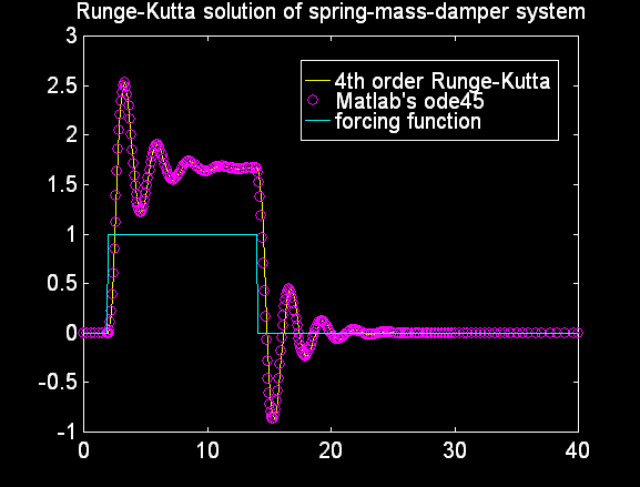
right hand side of second order ODE corresponding to a spring-mass-damper
Matlab code for Euler solution of a spring-mass-damper system excited by a square wave.
demonstration of a three solution methods to a first order ODE…
This program requires the function file: fcn1.m.
right hand side for spring-mass-damper ODE (see rk4ode2.m and rk4ada2.m)
right hand side for Van Der Pol’s ODE (see rk4ode2.m and rk4ada2.m)
adaptive 4th order Runge-Kutta (first order ODE)
adaptive 4th order Runge-Kutta (second order ODE) for spring-mass-damper or Van Der Pol’s equation (see functions rhs_smd.m and rhs_vdp.m)
4th order Runge-Kutta (first order ODE)
4th order Runge-Kutta (second order ODE) for spring-mass-damper or Van Der Pol’s equation (see functions rhs_smd.m and rhs_vdp.m)
Matlab code for Runge-Kutta solution of a spring-mass-damper system excited by a square wave. Two solutions are presented here:
Shooting Method demo code
Finite Difference demo code
Power method of solution for highest/lowest eigen value. Results of this program.
routine to take the Fourier transform of a signal and plot both the time and frequency domain representations. Typical use:
>> n = 100; % number of data points >> dt = 0.01; % spacing between samples >> t = 0:dt:(n-1)*dt; % time vector >> y = sin(2*pi*10*t); % 10 Hz sin wave >> fft_plot(y,dt); % plot of signal in time and frequency domain
examples of using MATLAB’s various matrix operators
plot a main or super title above a series of subplots
plotting function with labeling and titles
utility file to plot two functions simultaneously
area of an irregular closed contour
a simple program for digitizing an irregular shape
utility for on-screen control of view direction in 3D plots
an example of splitting long format strings in Matlab fprintf statements
Matlab_ExamplesBundle.zip Matlab Example Bundle

Copyright ©2017 - STI - Todos os direitos reservados